
What you'll build
A single-story steel frame with a concrete floor: the smallest model that still uses every part of the vfopro workflow. Once it runs, every larger model is the same steps repeated.
| Part | Definition |
|---|---|
| Plan | 20 ft × 20 ft, one story, 13 ft high |
| Columns | 4 × W14x90, one at each corner |
| Beams | W21x93 around the perimeter |
| Floor | 6 in concrete slab, 6 ksi, modeled as an elastic shell |
| Supports | Pinned at the base of each column |
| Floor behavior | Rigid diaphragm tying the four column-top nodes together |
vfopro starts every new model in kip · in · sec, so lengths are typed in inches: 20 ft is 240 and 13 ft is 156. Sections are always in inches, materials in ksi and area loads in psf, whichever unit system you choose.
Find your way around
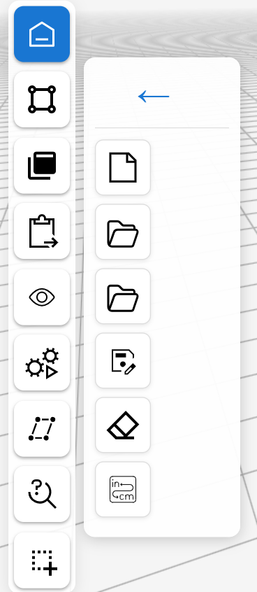
The rail down the left edge is how you move through the workflow. Each button opens a small panel of icons; hover over an icon to see its name.
Stage 1: Draw the geometry
Grid lines and a story level give you something to snap to, so every node lands exactly where you want it.
-
Start a new, empty model. Click Home on the rail, then the first icon, New Model.
You should see: a green “New model ready” message at the top right.While you are on the Home panel, the last icon is Unit System. Leave it on kip · in · sec, the first option.
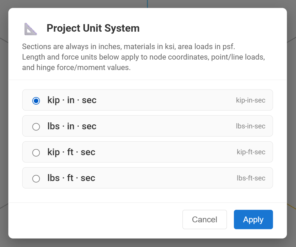
Home › Unit System. The default is kip · in · sec. -
Set up the grid lines. Click Create, then Grid System, then Grid Data. Fill in two lines in each table and leave the third row empty; empty rows are ignored.
- X Grids: tag
Aat0, tagBat240. - Y Grids: tag
1at0, tag2at240.
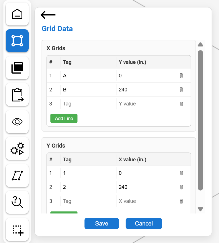
Create › Grid System › Grid Data. Click Save.
You should see: “Grid data saved successfully! X Grids: 2 Y Grids: 2”. - X Grids: tag
-
Set up the floor level. Click Create › Grid System › Story Data. The Base row (Ground Floor, elevation 0) is always there. In row 1, type the name
Level 1and the elevation156(13 ft), then click Save.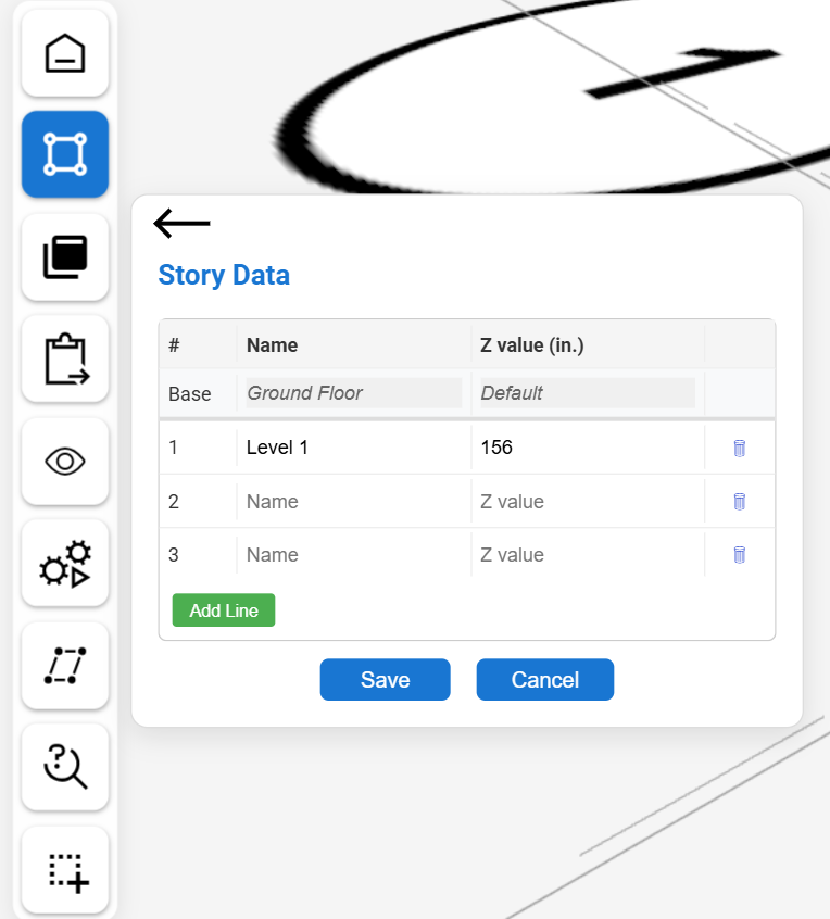
Create › Grid System › Story Data. You should see: “Story data saved successfully! … Total Stories: 2”. -
Switch to the 2D plan view at Level 1. Click Plan View in the bar at the top of the drawing area (the layers icon), then choose Level 1 (Elevation: 156).
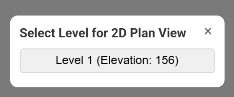
The plan opens close-up, so most of the 240 in grid is off screen. Scroll to zoom out and drag with the right mouse button to pan until you can see all four grid intersections (A1, B1, B2 and A2).
-
Draw a column at each grid intersection. In the toolbar at the bottom, click Column (or press C), then click each of the four intersections. Green snap markers and a readout show that the pointer has locked onto the intersection.
A column runs from the level below up to the level you are viewing, so vfopro also creates a node directly under each one at elevation 0.
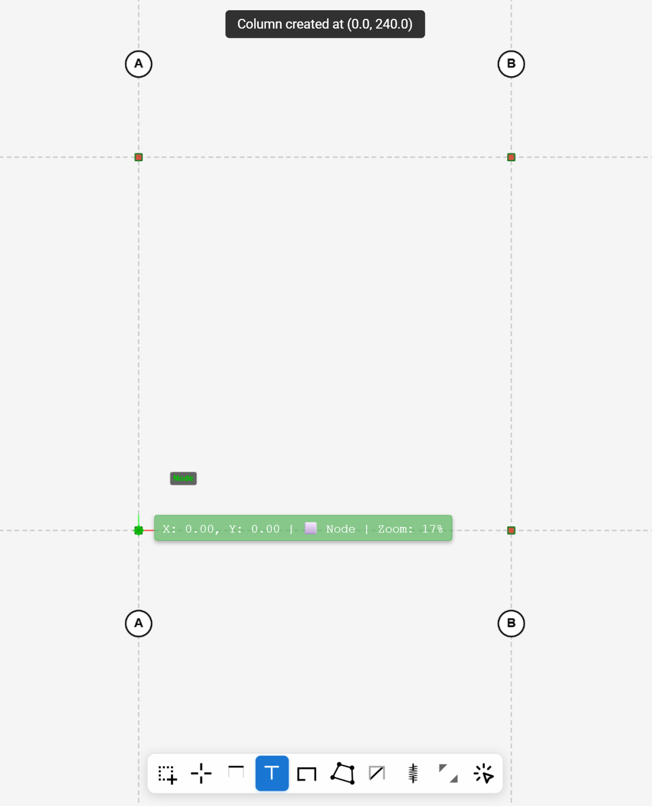
Plan view, Level 1. Each small square marks a column. You should see: “Column created at (…)” after each click, four times in all. -
Draw the perimeter beams. Click Beam (or press B). Click A1, then B1, B2, A2 and back to A1. Each click after the first draws a beam from the previous point. Right-click to stop drawing.
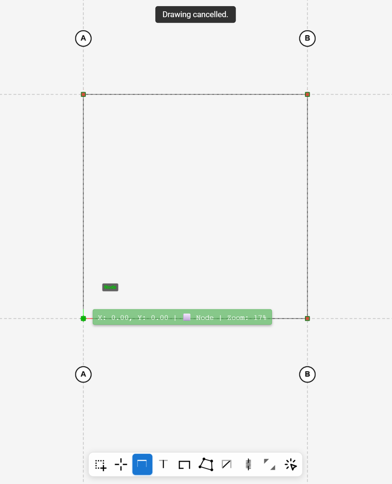
Four beams around the square. “Drawing cancelled.” only means the right-click ended the chain. -
Switch to the 3D view. Click 3D View (the cube icon, next to Plan View). Scroll to zoom out and drag to orbit until the whole frame is in view.
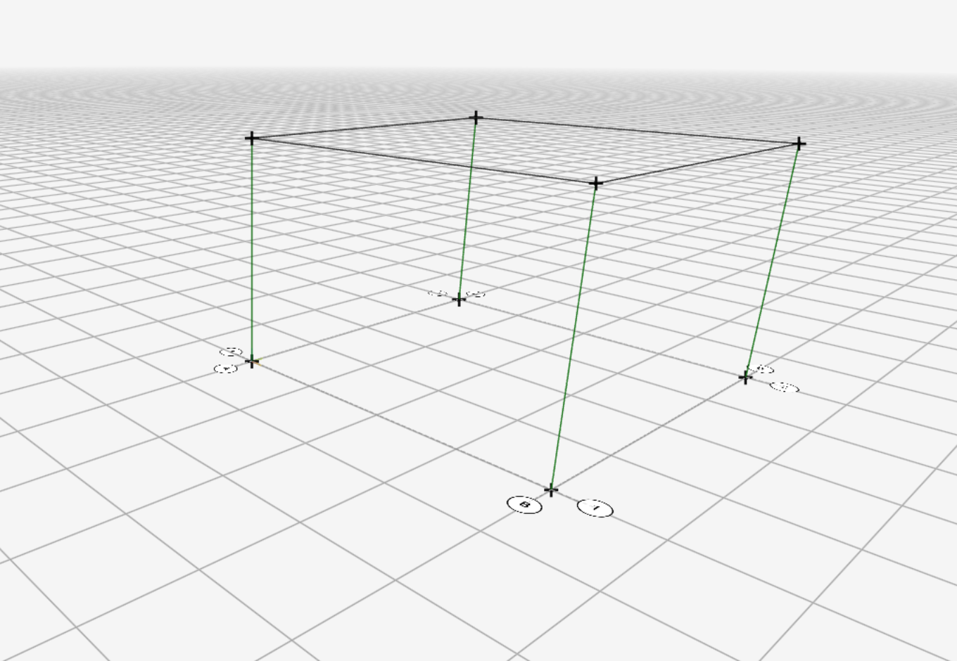
Four columns and four beams in 3D. -
Draw the floor as a shell element. Click Create › Elements and choose the last icon, Quad. Then click the four nodes at the top of the columns, going around the square in order.
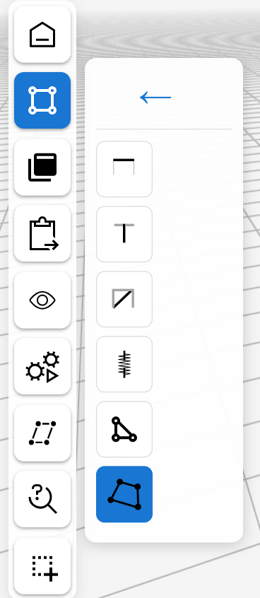
Create › Elements. 1 is the Quad tool. 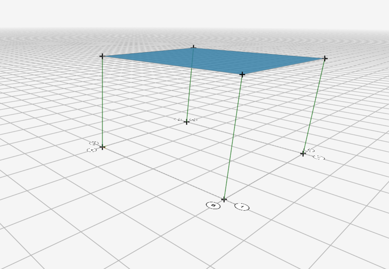
The floor appears as a blue surface. Click the back arrow at the top of the Elements panel to put the Quad tool away.
Checkpoint: 4 columns, 4 beams and 1 floor element. Hover over one of them and vfopro shows its type, ID, section and material (the section is still Unassigned).
Stage 2: Sections, supports and the diaphragm
The geometry has no properties yet. First you define the sections, then you assign them, along with the supports and the diaphragm, to the parts you select.
-
Define the column, beam and shell sections. Click Define › Sections.
Column and beam: under Frame, click the first icon (Linear elastic section properties), then Steel W. Fill in the form, then click Save.
- Column: Name
W14x90, MaterialSteelA36, AISC ShapeW14X90. - Beam: Name
W21x93, MaterialSteelA36, AISC ShapeW21X93.
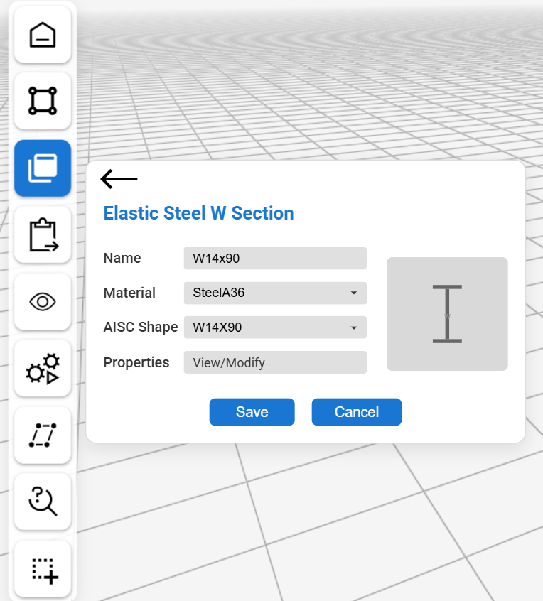
Define › Sections › Frame › Steel W. The form stays open after you save. Your section is already stored; click Cancel to close the form.
Slab: under Shell, click the icon (Linear elastic membrane plate section). Enter Section Name
Slab6in, MaterialConc6ksiand Thickness (t)6, then Save.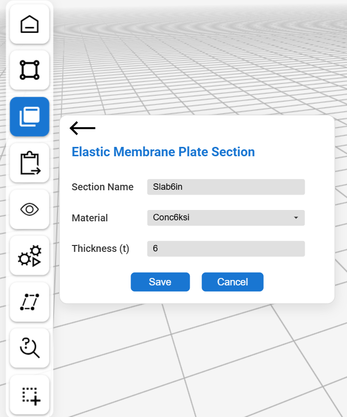
Define › Sections › Shell. You should see: “Section "W14x90" created successfully” (and likewise for the other two). This guide uses vfopro’s built-in materials,SteelA36andConc6ksi. - Column: Name
-
Apply the sections. Assign works on whatever is selected, so select first. Two selection rules cover everything in this guide:
- Select (the last button on the rail) turns selection on. Click an element to add it, or drag a box to select everything the box touches, nodes included.
- Press Esc once to leave selection, and again to clear the selection.
a. Beams and slab. Click Select and drag a box around the whole frame. Green highlights show what is selected.
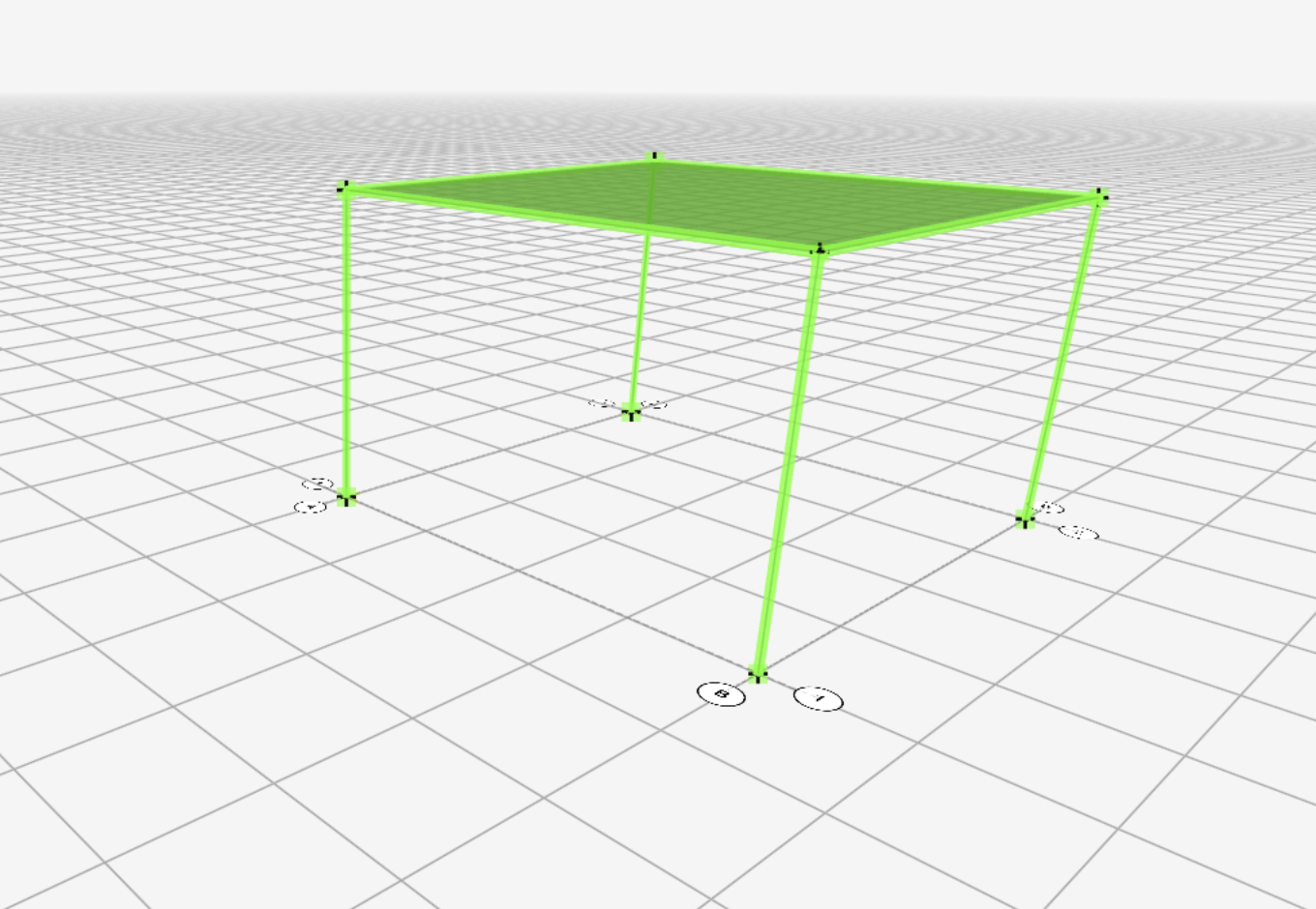
Everything selected. Click Assign › Frame › Section, click the W21x93 card and click Apply. This gives every frame element the beam section for now; the next part fixes the columns. Then click Assign › Shell › Section, click Slab6in and Apply. Only the floor takes the shell section.
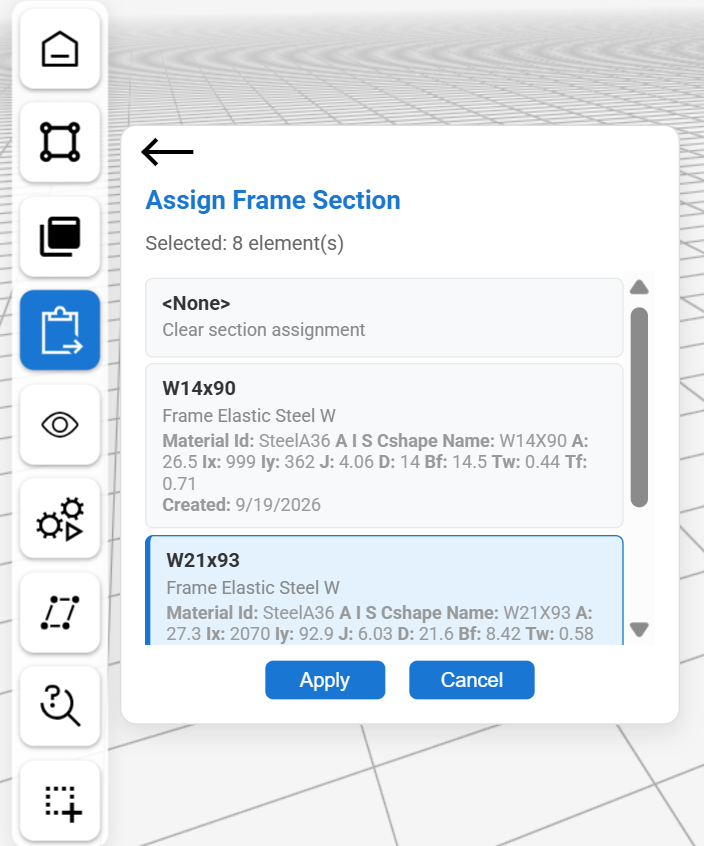
Assign › Frame › Section lists your sections. Click a card, then Apply. b. Columns. Press Esc twice, click Select, and drag a box around the bottom of the frame, below the beams and floor. It catches the four columns and the four base nodes.
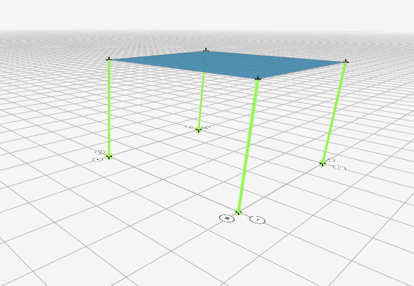
The four columns and their base nodes. Click Assign › Frame › Section, click W14x90 and Apply.
You should see: “Successfully assigned section "W14x90" to 4 frame element(s).” Hover over a column, a beam and the floor to confirm each shows the right section. -
Pin the column bases. The base nodes are still selected from the last step. Click Assign › Node › Restraints, tick UX, UY and UZ (translations fixed, rotations free) and click Apply.
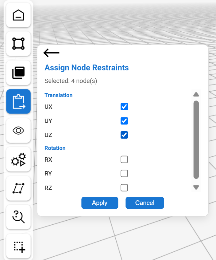
Assign › Node › Restraints. Pin = UX, UY, UZ. You should see: a red support symbol at the base of each column. -
Make the floor a rigid diaphragm. First define it: click Define › Constraints › Diaphragm, name it
Level1_Diaphragm, leave Diaphragm Axis on Z (a horizontal floor) and click Save.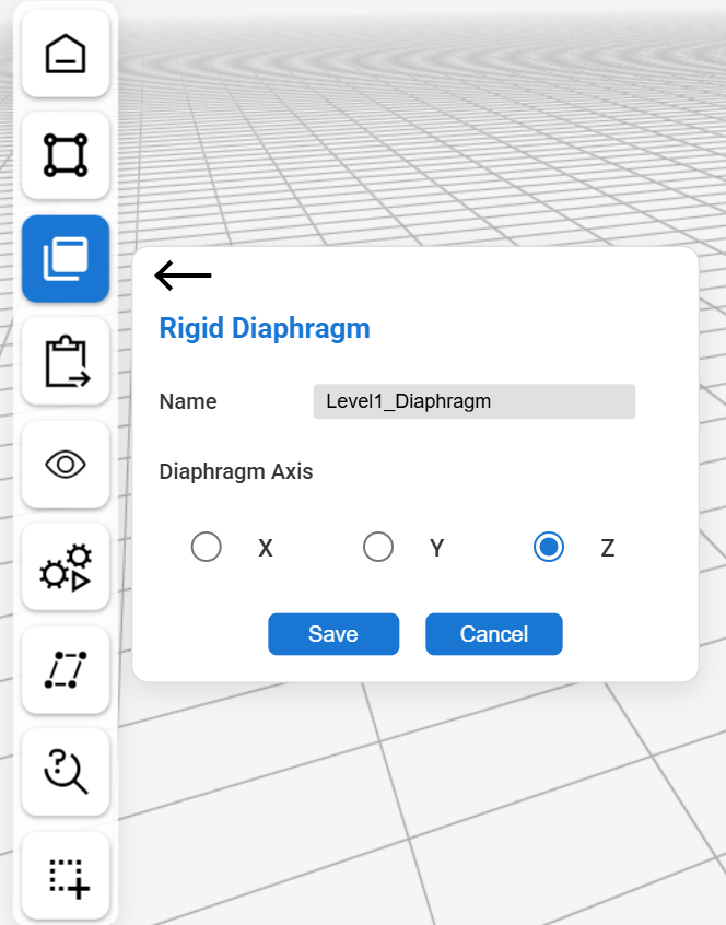
Define › Constraints › Diaphragm. Then assign it to the column-top nodes. Press Esc twice, click Select and drag a box around the top of the frame. Click Assign › Node › Constraints › Rigid Diaph., choose Level1_Diaphragm and click Apply.
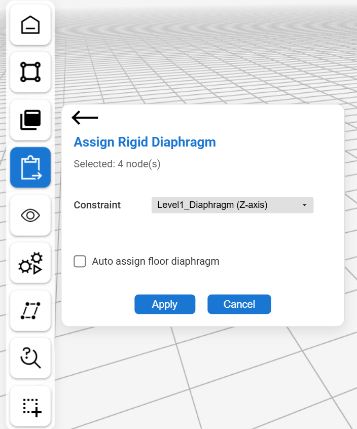
Assign › Node › Constraints › Rigid Diaph. You should see: “Selected: 4 node(s)” at the top of the panel. If it says a different number, close the panel, redo the box selection and try again.
Stage 3: Load cases and analysis
-
Look at the gravity load case. vfopro starts every model with two load cases: Modal (mode shapes) and Dead, a nonlinear static case that applies the Dead load pattern at scale factor 1. That pattern applies the self-weight of the model at a multiplier of 1, so Dead is your gravity case and you do not need to create another. See them under Define › Loads › Cases › Show All.
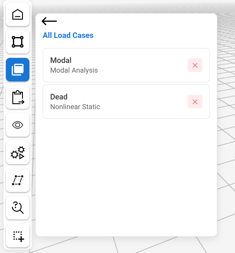
Define › Loads › Cases › Show All. -
Save the model, check it, and run the analysis. vfopro writes the analysis files next to your model file, so the model has to be saved first. Click Home › Save As (the fourth icon), choose a folder and a name such as
portal-frame, and click Save. The model name appears at the top left of the window.Click Analysis on the rail. The table lists your load cases; leave Modal and Dead ticked.
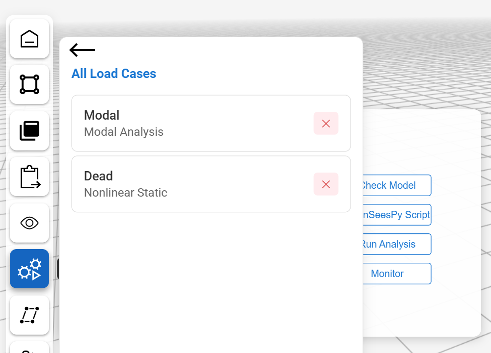
The Analysis panel. Click Check Model first. It scans the model for problems before you spend time on a run.
You should see: “No issues found”. If Check Model warns that it could not verify mass because no model file is loaded, save the model and check again.Click Run Analysis. Progress appears in the terminal below the table and in the convergence monitor. This small model finishes in a few seconds.
You should see: Complete next to both Modal and Dead in the table, and “All analyses complete” followed by “Process completed with exit code: 0” at the end of the terminal. The convergence monitor shows Dead stepping to 100/100 with a residual near zero.
Stage 4: View your results
-
Read the natural periods. The Modal case finds the frame's mode shapes and their periods. In the Analysis panel, scroll the terminal up to “Calculated modal periods”.
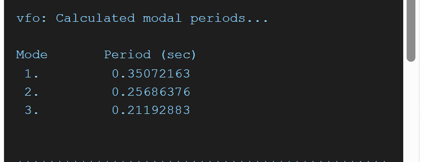
The modal periods in the Analysis terminal. You should see: three periods of about 0.351 s, 0.257 s and 0.212 s.About the solver warningHigher up in the terminal you will see “ARPACK eigen solver failed (the model has only 3 dynamic DOFs for 4 requested eigenvalues). Switched to fullGenLapack solver.”, followed by a red note from OpenSees that
fullGenLapackis slow. That is expected for this model: with the rigid diaphragm it has only three degrees of freedom that carry mass (two translations and one twist), too few for the default ARPACK solver, so vfopro switches to the dense solver by itself. Nothing to change; it takes a fraction of a second here. -
Show the mode shapes. Click Post, the seventh button on the rail, to open Post Processing. With Mode selected, choose 1 in its list and click OK. This run computed three modes, so pick 1, 2 or 3.
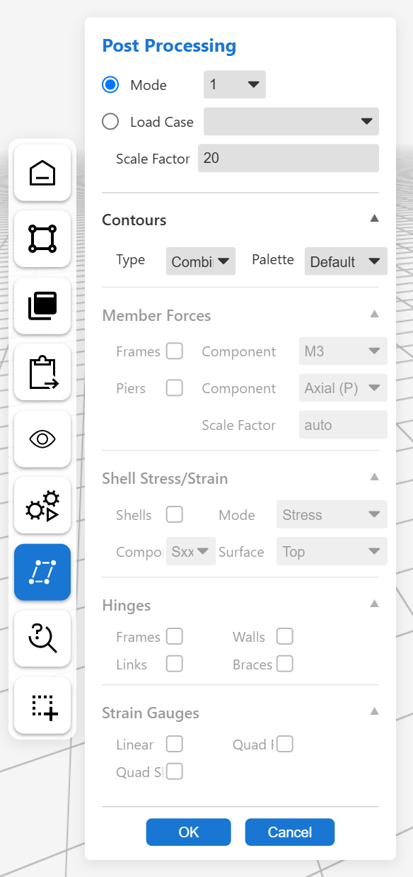
The Post Processing panel. The frame appears in its deformed shape, drawn over a light grey outline of the undeformed frame. The Scale Factor (20 by default) exaggerates the movement so you can see it; it does not change the results. Repeat with modes 2 and 3.
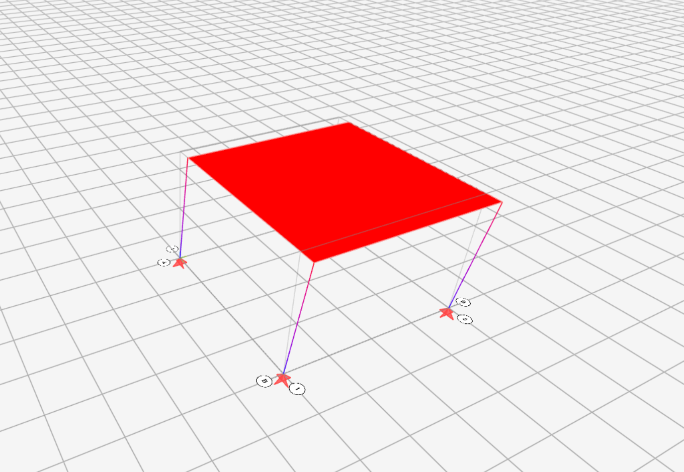
Mode 1, T = 0.351 s. 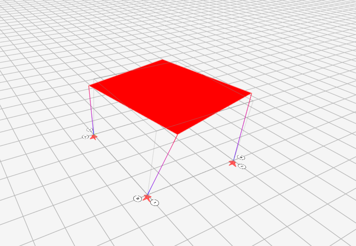
Mode 2, T = 0.257 s. 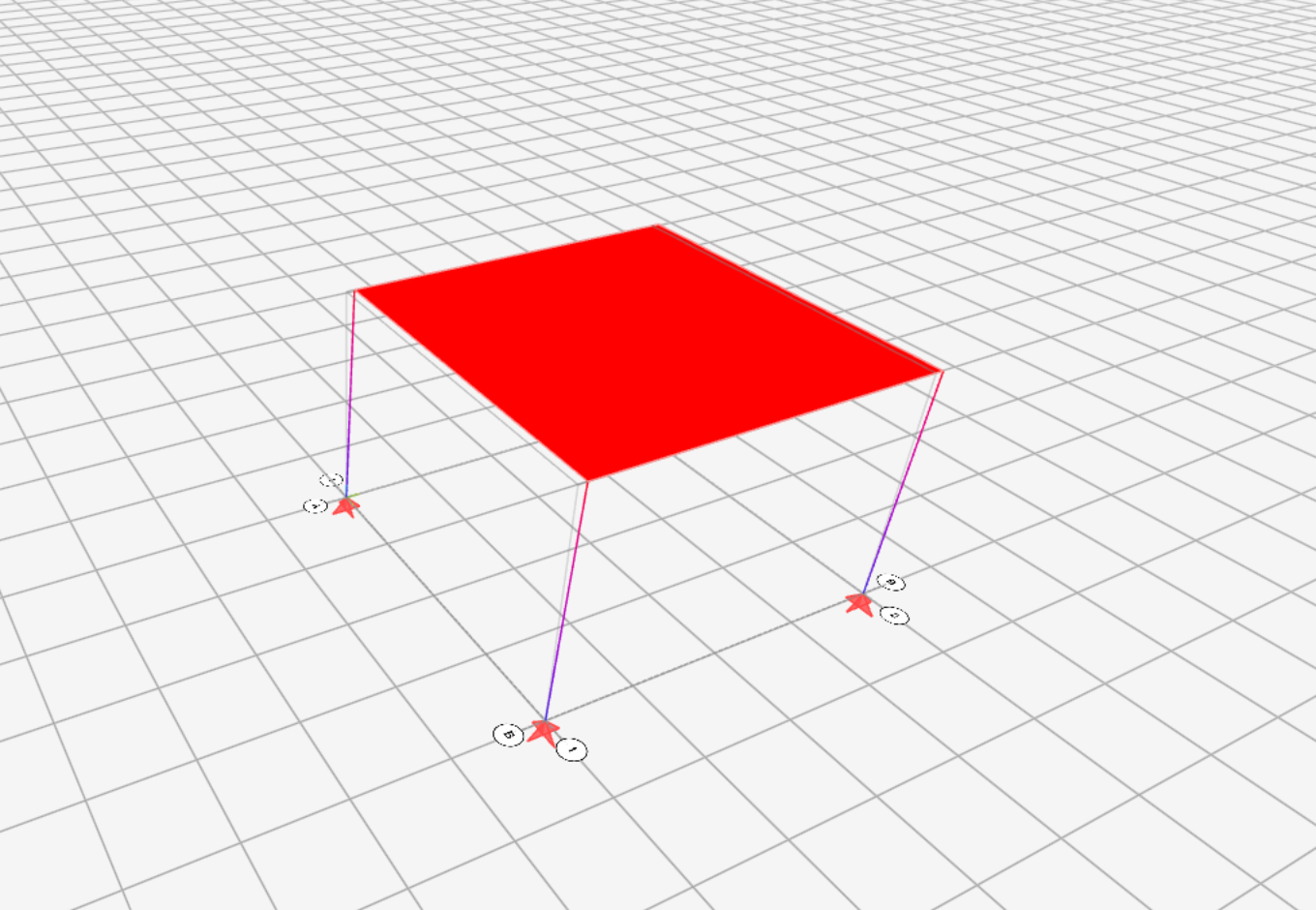
Mode 3, T = 0.212 s. You should see: mode 1 slides the floor along X, mode 2 twists it about the vertical axis, and mode 3 slides it along Y. In all three the floor moves as one rigid piece, because of the diaphragm. -
Animate a mode. When a result is on screen, an Animation bar appears at the bottom of the view. Click Play/Resume to watch the frame move through the mode shape, Pause to hold it and Stop to return to the start.

The Animation bar. -
Show contours. Under Contours in the Post Processing panel, Type chooses what to colour by: Combined (the default), X, Y, Z or None. Palette chooses the colours: Default, Rainbow, Thermal or Cool-Warm. Choose mode 2, set Type to X and Palette to Rainbow, then click OK.
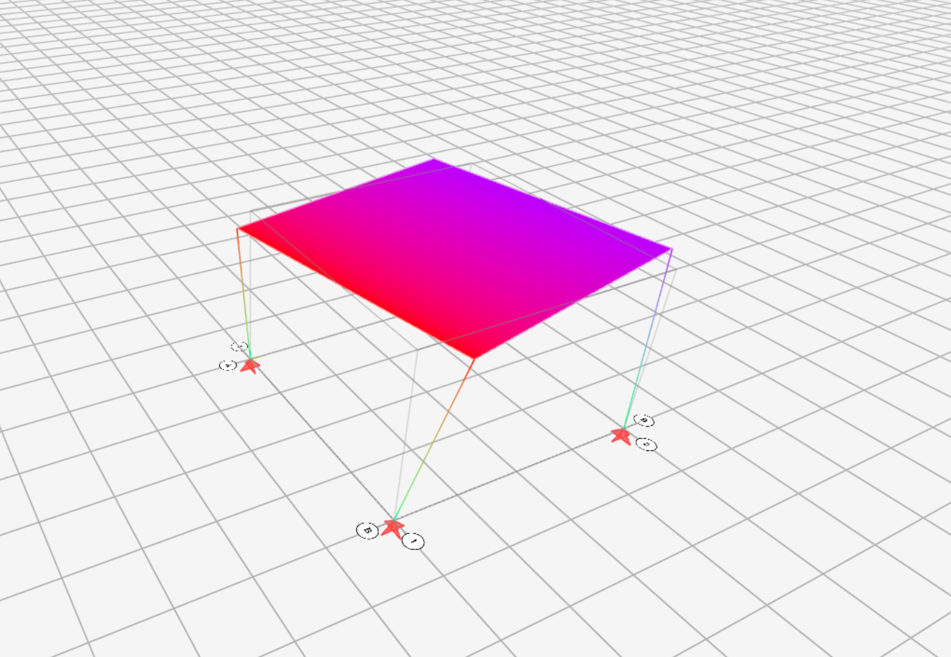
Mode 2, X contours, Rainbow palette. You should see: colours that run across the floor from one edge to the opposite edge. In a twist, one side of the floor moves in +X while the other moves in −X. Try the same settings on mode 1: the floor is a single colour, because everything on it moves the same amount. -
Render the frame forces. Open Post Processing again. Select Load Case and choose Dead in its list. For a clean view, set Type under Contours to None. Under Member Forces, tick Frames, choose M3 as the Component (the others are Axial, V2, V3, M2 and T) and click OK.
vfopro applies the Dead case in 100 load steps and starts on the first, when only 1% of the load is on the frame, so the diagram is barely visible. Click Play/Resume on the Animation bar to watch it grow as the load is applied, and Pause to hold a step.
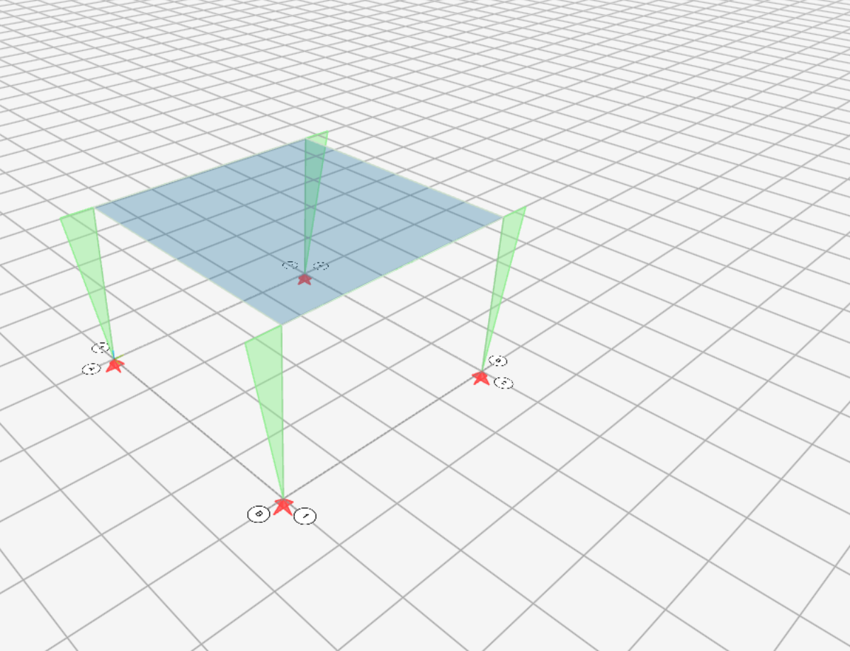
M3 for the Dead case near the last load step. You should see: a green triangle along each column that shrinks to nothing at the base and is largest at the top. A pinned base cannot resist moment, so the diagram has to reach zero there; if it does not, the restraints were not assigned to the base nodes.
What's next
You now know the whole modeling loop: grid and story, draw, define, assign, analyze. Next, let the AI assistant do the repetitive parts, or move on to a performance-based assessment.
Last updated September 20, 2026 · applies to vfopro 20260918.0.0 or later